I've got three big spreadsheets with around 80 tabs each. Two of them have identical workbook names, the only difference being the year. The tab names are also identical, and are all a 3 digit number that corresponds to a department code in our accounting software.

What I am trying to do is in my main file, use a vlookup formula to reference those two other files and pull in actual revenue and expenses. My lookup will be the same column set in the identical workbooks. B through H columns. They also all start at row 10. So my current formula looks like:

=vlookup(A10,'[BudgetExport 2025 Actuals.xlsx]359'!$B1$12;$H$106,7,false)

Is there a way to embed a formula to replace the '[BudgetExport 2025 Actuals.xlsx]359' with something that reads two cells in my current workbook and put the year and tab name in there where it has 2025 and 359'. I've tried concatenate, but that doesn't seem to work.

In Summary, starting at row 10 in each of my tabs I want a formula that references A10 down through A105 or so, and is looking up values from each of the other two workbooks that can quickly read the year and tab name. Not sure if this is possible, but if I could write one formula and copy/paste that down my rows of data instead of manually typing a vlookup and clicking over to the other two workbooks it would save a ton of time.

6 ...

Report Post

Posted by Korkstand

Member since Nov 2003

29132 posts

Posted on 7/29/26 at 12:58 pm to TU Rob

My response to your exact question is I would feed the file to AI and have it write formulas for what you want, then verify.

But to really solve your problem, which as I understand it is

quote:
save a ton of time

I would put this data in a database and write queries. AI can plop out a pretty frontend for it too if you want.

1 ...

Report Post

Posted by TU Rob

Birmingham

Member since Nov 2008

13541 posts

Posted on 7/29/26 at 1:42 pm to Korkstand

Yeah i've asked AI on how to reference the other file and sheet name, but trying their indirect formula keeps giving me formula errors. This is an exercise I only do once a year for our budget, so don't feel like wasting too much time down a rabbit hole of databases. Was hoping a simple formula using file names and sheet names would work.

2 ...

Report Post

Posted by Korkstand

Member since Nov 2003

29132 posts

Posted on 7/29/26 at 1:57 pm to TU Rob

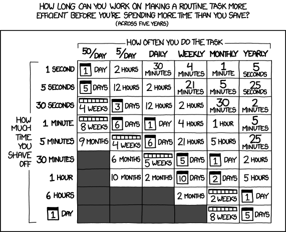
I don't think I can help without having the actual file for testing. Sorry.

But if I did have the file I would still use AI to write a script to dump the sheets to sqlite and write queries. Because I just know I would come back next year and have some kind of issue with the excel sheets.

0 ...

Report Post

Posted by mdomingue

Lafayette, LA

Member since Nov 2010

48372 posts

Posted on 7/29/26 at 2:13 pm to TU Rob

Substitue Y1 as the cell with the year and Z1 as the cell with the Tab name; try this formula and see if it works for you

=vlookup(A10,INDIRECT(CONCAT('[BudgetExport ",Y1,"Actuals.xlsx]",Z1,"'!$B1$12;$H$106",7,false)

ETA: Y1 & Z1 will need to be $Y$1 and $Z$1 if you want all those calls to reference a single pair of cells in the spreadsheet

This post was edited on 7/29/26 at 2:17 pm

0 ...

Report Post

Posted by broadhead

Member since Oct 2014

2601 posts

Posted on 7/29/26 at 4:05 pm to TU Rob

Feed it to co-pilot and have it fix it. If you're company doesn't pay for it then buy it your self.

0 ...

Report Post

Posted by LemmyLives

Texas

Member since Mar 2019

17354 posts

Posted on 7/29/26 at 6:45 pm to TU Rob

I agree with Kork. Explain what you need to ChatGPT the way you did here. Check the output with a high level of scrutiny. Give it feedback, repeat as necessary.

0 ...

Report Post

Posted by CPA Yung Boi

Member since Apr 2026

200 posts

Posted on 7/29/26 at 9:56 pm to TU Rob

I’d put this in alteryx and add the sheet names as a field and then just join them.

But assuming you can’t do that just macro the sheets into a database format and do a vlookup

0 ...

Report Post

Posted by Ingeniero

Baton Rouge

Member since Dec 2013

23466 posts

Posted on 7/30/26 at 8:32 pm to TU Rob

There have been some good answers already. Throwing another option out, I've used Phind AI to write complicated Excel formulas for me. You can explain it exactly how you did in your OP and it'll give you a nice neat output and even show you flow charts on why things are arranged or nested a certain way

0 ...

Report Post

Posted by Breauxsif

Member since May 2012

23035 posts

Posted on 7/31/26 at 9:38 am to TU Rob

What you are trying to do is possible, but it requires a specific function called INDIRECT, which turns a text string into a live cell reference. Standard concatenation (&) alone won't work because Excel treats the result as plain text rather than an active formula reference unless INDIRECT wraps it.

Try this:

=VLOOKUP(A10, INDIRECT("'[BudgetExport " & $Z$1 & " Actuals.xlsx]" & $Z$2 & "'!$B$10:$H$106"), 7, FALSE)

$Z$1 and $Z$2: These point to your variable cells for the year and department code, allowing you to drag the formula down safely using absolute anchoring like $ where appropriate.

The INDIRECT Argument:
"'[BudgetExport " & $Z$1 & " Actuals.xlsx]" & $Z$2 & "'!$B$10:$H$106"

This stitches your text pieces together into exactly what Excel needs to read. BudgetExport 2025 Actuals.xlsx]359'!$B$10:$H$106.

Furthermore, the VLOOKUP Execution:
INDIRECT wraps that text string so Excel evaluates it as a real table range, and the VLOOKUP searches column A10 inside it, returning the value from the 7th column (H).

1 ...

Report Post

Posted by dtett

Jiggacity

Member since Oct 2018

563 posts

Posted on 7/31/26 at 11:53 am to Breauxsif

Another thing, stop using vlookup. Use Xlookup or lean to use index match. Both are more efficient than vlookup.